Examples
This page has some examples of using the Calcam API. It is not meant to demonstrate all API features exhaustively, but gives some examples of simple use cases and workflows; for more complete details of the API features please refer to the other API documentation pages.
Mapping a magnetic field line on to an image
We start with an image of a MAST plasma on to which we want to overlay a magnetic field line, which we will assume is saved as image.png in the current directory. We also have a Calcam calibration for that image stored in the file mycalib.ccc, which for convenience we assume is also saved in the current directory. Finally, we have a .csv file containing a set of 3D coordinates of points along a magnetic field line (generated using a field line tracing tool), with each row of the file containg X,Y,Z coordinates of a single point.
We can plot the field line on top of the image with the following code:
import calcam
import numpy as np
import cv2
import matplotlib.pyplot as plt

# Load the image using OpenCV
cam_image = cv2.imread('image.png')

# Load the field line coordinates
fieldline_3d = np.loadtxt('fieldline.csv',delimiter=',')

# Load the calcam calibration
cam_calib = calcam.Calibration('mycalib.ccc')

# Project the field line coordinates to image coordinates using calcam.
# Note: the [0] index here is because this is a single sub-view image and
# we want the image coordinates for sub-view #0.
fieldline_2d = cam_calib.project_points(fieldline_3d)[0]

# Plot the projected coordinates on the image.
plt.imshow(cam_image)
plt.plot(fieldline_2d[:,0],fieldline_2d[:,1])
plt.show()
This results in the figure below:
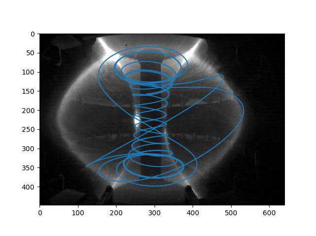
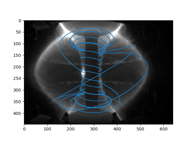
Note that the parts of the field line hidden behind the centre stack are still visible, which looks strange. To only show the parts of the field line which are not hidden behind parts of the machine, we can modify the above code to also load the MAST CAD model and check which points are hidden from the camera by the CAD geometry:
import calcam
import numpy as np
import cv2
import matplotlib.pyplot as plt

# Load the image using OpenCV
cam_image = cv2.imread('image.png')

# Load the field line coordinates
fieldline_3d = np.loadtxt('fieldline.csv',delimiter=',')

# Load the calcam calibration
cam_calib = calcam.Calibration('mycalib.ccc')

# Load the MAST CAD model
mast_machine = calcam.CADModel('MAST')

# Project the field line coordinates to image coordinates using calcam.
# This time, check for occlusion of the points by the CAD model.
# Note: the [0] index here is because this is a single sub-view image and
# we want the image coordinates for sub-view #0.
fieldline_2d = cam_calib.project_points(fieldline_3d,check_occlusion_with=mast_machine)[0]

# Plot the projected coordinates on the image.
# Occluded points now have np.nan in their coordinates, so MatPlotLib skips them
# and we see only the points not hidden behind bits of CAD model.
plt.imshow(cam_image)
plt.plot(fieldline_2d[:,0],fieldline_2d[:,1])
plt.show()
Which results in the following figure:
Rendering: camera view wireframe
For this example, we start with a Calcam calibration for a MAST camera, and we want to render a wireframe version of the MAST CAD model which aligns with the camera image. This might be used, for example, to use as an overlay on a plasma image to give context to the image. We can do this with the following code:
import calcam
import matplotlib.pyplot as plt

# Load the calcam calibration
cam_calib = calcam.Calibration('mycalib.ccc')

# Load the MAST CAD model and set it to be bright red wireframe
mast_machine = calcam.CADModel('MAST')
mast_machine.set_wireframe(True)
mast_machine.set_colour((1,0,0))

# Render the image to produce the array rendered_im
# Also save as an image file "wireframe.png"
rendered_im = calcam.render_cam_view(mast_machine,cam_calib,filename='wireframe.png')

# Show the rendered image using matplotlib
plt.imshow(rendered_im)
plt.show()
This results in the following plot:
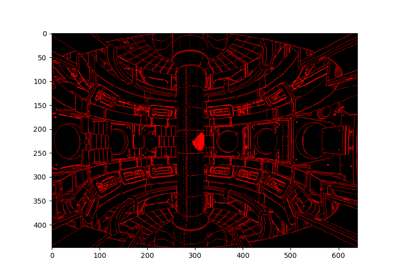
and also the same image saved to the file wireframe.png.
Ray casting
Imagine we have an IR image from a first wall monitoring camera which shows some unusual event at pixel coordinates (100,250). We might want to get the 3D coordinates on the CAD model corresponding to this pixel to tell us where exactly this event took place. We could do this by ray-casting that particular pixel:
import calcam

# Load the calibration
cam_calib = calcam.Calibration('my_calibration.ccc')

# Load the CAD model
jet_machine = calcam.CADModel('JET')

# Do the ray cast to find the sight-line / CAD model intersection coordinates
raydata = calcam.raycast_sightlines(cam_calib,jet_machine,x=100,y=250)

# The coordinates at the wall are contained in the raydata's ray_end_coords array.
coords = raydata.ray_end_coords[0,:]
The 3-element array coords will then contain the \(X,Y,Z\) coordinates, in metres, of where the event of interest appened.
Alternatively, we could ray cast every pixel on the detector and then find the coordinates from whiever one(s) we want afterwards:
# Do the ray cast to find the sight-line / CAD model intersection coordinates
raydata = calcam.raycast_sightlines(cam_calib,jet_machine)

# The coordinates at the wall are contained in the raydata's ray_end_coords array.
coords = raydata.ray_end_coords[250,100,:]

# While we're at it, save the raydata in case we need it again later
raydata.save('my_raydata.nc')
Tomography Geometry Matrices
For this example, we assume we already have a set of saved raydata relating to a camera we want to tomographically invert. For the purposes of this example we imagine it is a divertor camera on MAST, which can see Z heights up to about -0.6m in its field of view. To make the geometry matrix, we do this:
import calcam
import matplotlib.pyplot as plt
import numpy as np

# Note that including "if __name__ == '__main__' is actually important here;
# because the geometry matrix calculation uses multiprocessing, this
# python file will be imported in each child thread and if we omit this
# if statement, lots of bad things will happen.
if __name__ == '__main__':
        # Load the raydata (see previous example for how to generate raydata)
        raydata = calcam.RayData('my_raydata.nc')

        # Make a grid with 1cm grid cells in the poloidal plane on to which to invert.
        # This will use the wall contour from the 'MAST' CAD model
        grid = calcam.gm.squaregrid('MAST',cell_size=1e-2,zmax=-0.6)

        # We can plot the grid to check it looks OK:
        grid.plot()
        plt.show()

        # Now we have our grid and raydata, we can make a geometry matrix:
        geom_mat = calcam.gm.GeometryMatrix(grid,raydata)

        # We probably want to save it, so we can use it to invert any images from this camera.
        geom_mat.save('my_geom_mat.npz')

        # If we want to use MATLAB to do the inversions, we can also save it in MATLAB format:
        geom_mat.save('my_geom_mat.mat')

        # If we need to make the matrix smaller to make the inversion computation easier,
        #  we can tell it to bin the camera image, e.g. in 4x4 pixel blocks:
        geom_mat.set_binning(4)

        # We could also inspect the number of sight-lines passing through each grid cell,
        # to get an idea of the camera's coverage of the reconstruction domain.
        coverage = geom_mat.get_los_coverage()
        geom_mat.grid.plot(coverage,cblabel='Number of sight-lines')
        plt.show()
Now let’s imagine we have an image from the camera in a (height x width) NumPy array called image, which we want to invert. The actual solver for \(Ax = b\) to do the inversion is beyond the scope of Calcam, so let’s assume your sparse matrix solver of choice is a function with call signature x = my_solver(A,b), where x will be a 1D vector containing the result, A is the geometry matrix and b is the input data vector. We would then do the tomographic inversion like so:
# Re-format the camera image in to a 1D vector ready for inversion.
# Note: if we have binning or pixel exclusion set up in the geometry matrix,
# this takes care of all that for us (we just feed it the raw camera image).
data_vec = geom_mat.format_image(image)

# Call our sparse matrix solver of choice
x = my_solver(geom_mat.data, data_vec)
We can then visualise the results and / or extract them for further analsys. Note that it is not straightforward to directly get the inversion results at a given \(R,Z\) position directly from x, since the order of veluaes in x corresponds to the order of the cell indexing in the grid, which can be arbitrary and depends on how the grid was constructued. We therefore need to use the grid’s interpolate() method to do this:
# Have a look at the results!
geom_mat.grid.plot(x)
plt.show()

# Now let's say we want to get the inversion results
# along a slice at Z = -1.3m, for R from 0.3 -> 1.2m
r_coords = np.linspace(0.3,1.2,90)
z_coords = np.zeros(Rslice.shape) - 1.3

result_along_slice = geom_mat.grid.interpolate(x,r_coords,z_coords)
Camera Movement Correction
Let’s say we have a good calibration, and we have a calcam.Calibration object for it in my_calib. We also have an image from the same camera some time later when the camera has moved, stored in a Numpy array called moved_im. We can then try to determine the correction to align the moved image with the calibration by:
mov = calcam.movement.detect_movement(my_calib, moved_im)
Alternatively, we can determine the camera movement manually using the GUI by:
mov = calcam.movement.manual_movement(my_calib, moved_im)
Now we have a movement correction object, we can use it to warp the new image so it aligns with the calibration:
corrected_image, mask = mov.warp_moved_to_ref(moved_im)
The array corrected_image then contains the image warped to align with the calibration, while mask is an array the same size as the image containing True where a pixel in the warped image contains real image data, and False if the corresponding pixel is outside the border of the actual data.
Alternatively, we could create an updated calibration object accounting for the camera movement:
updated_calib = calcam.movement.update_calibration(my_calib,moved_im,mov)
We can also save the movement correction for use again later, and load it back from a file:
mov.save('my movement correction.cmc')
mov_loaded = calcam.movement.MovementCorrection.load('my movement correction.cmc')